URLit.me Blogs

PySpark — JDBC Predicate Pushdown

SQL Data sources are the well known data sources for transactional systems. Spark has out of the box capability to connect with SQL sources with help of Java Database Connectivity aka JDBC drivers and its as easier as reading from File data sources.

We are going to use the simplest SQLite database to check how can we optimize the performance of reads. Will also dig into explain plans to understand how Spark optimizes it for performance benefits.

So, without delay lets jump into action.

In order to read from SQLite database we would need to load the JBDC jar as library in our notebook. Now, this step is important.

Checkout below how the SparkSession is created to import the jar as library on runtime in notebook.

# Create Spark Session
from pyspark.sql import SparkSession
spark = SparkSession \
    .builder \
    .appName("Predicate Pushdown") \
    .config('spark.jars.packages', 'org.xerial:sqlite-jdbc:3.39.3.0') \
    .master("local[*]") \
    .getOrCreate()
spark

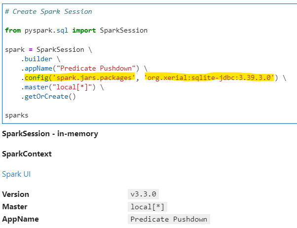
Now, since we imported the JDBC library successfully, lets create our Python decorator for performance measurement. We will use “noop” format for performance benchmarking

# Lets create a simple Python decorator - {get_time} to get the execution timings
# If you dont know about Python decorators - check out : https://www.geeksforgeeks.org/decorators-in-python/
import time
def get_time(func):
    def inner_get_time() -> str:
        start_time = time.time()
        func()
        end_time = time.time()
        return (f"Execution time: {(end_time - start_time)*1000} ms")
    print(inner_get_time())

Define the JDBC data source parameters

# Set up to read from JDBC SQLite database
driver: str = "org.sqlite.JDBC"
db_path: str = "dataset/jdbc/demo-sqlite.db"
jdbc_url: str = "jdbc:sqlite:" + db_path
table_name: str = "sales_csv"

Lets check the data from the SQLite DB for validation. Keep a note on timings.

# Lets read the SQLite table using JDBC driver and validate the data
df = spark \
    .read \
    .format("jdbc") \
    .option("driver", driver) \
    .option("url", jdbc_url) \
    .option("dbtable", table_name) \
    .load()
df.printSchema()
df.show(10, False)

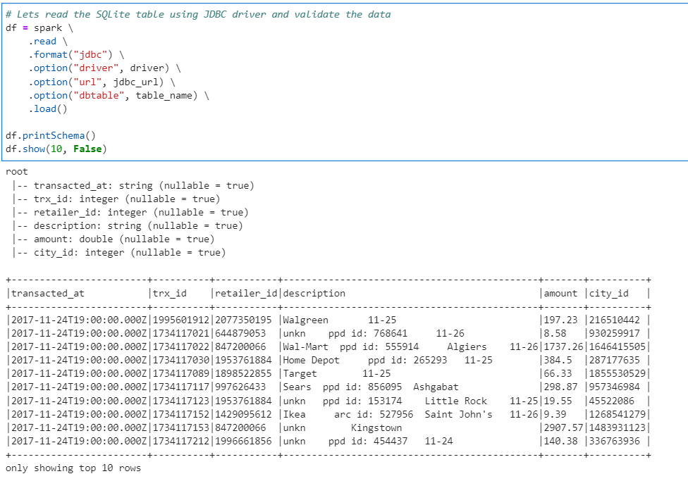
Without any Predicate: First we read the data without any filters or predicates specified.

# Checking the performance for Full read without any Predicate Pushdown
@get_time
def x():
    df_full = spark \
    .read \
    .format("jdbc") \
    .option("driver", driver) \
    .option("url", jdbc_url) \
    .option("dbtable", table_name) \
    .load()
    
    df_full.write.format("noop").mode("overwrite").save()
    df_full.explain(True)

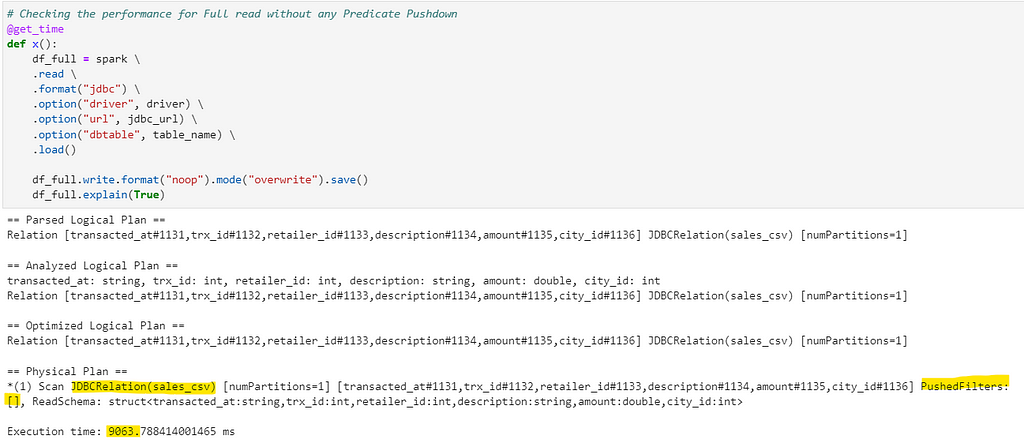
The Physical query in explain plan shows no filters being pushed while reading the data from database.

With Predicate Pushdown: We push our required filters directly to database while reading the data. In this case we will filter based on city_id

# Checking the performance for Predicate Pushdown
@get_time
def x():
    df_filtered = spark \
    .read \
    .format("jdbc") \
    .option("driver", driver) \
    .option("url", jdbc_url) \
    .option("dbtable", table_name) \
    .load() \
    .filter("city_id = 216510442")
    
    df_filtered.write.format("noop").mode("overwrite").save()
    df_filtered.explain(True)

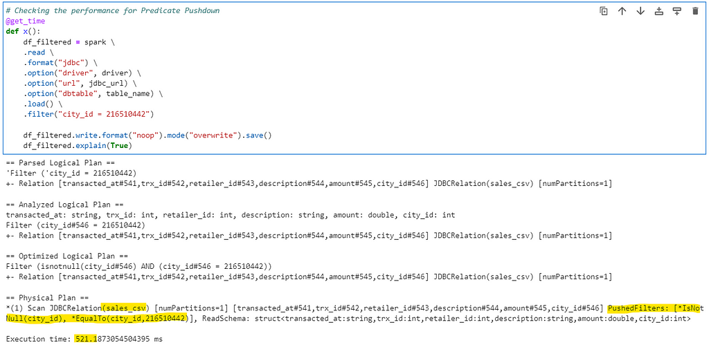
Spark optimizes the Physical plan and pushes the filter directly to database while reading the data.

With Pushed Queries: We can even push database queries to optimize the performance further more. Consider an aggregation based on a city_id

# We can even push down Queries for perfomance benifits
pushDownQuery = """(select city_id, count(1) as cnt from sales_csv group by city_id) as sales_csv"""
@get_time
def x():
    df_filtered = spark \
    .read \
    .format("jdbc") \
    .option("driver", driver) \
    .option("url", jdbc_url) \
    .option("dbtable", pushDownQuery) \
    .load()
    
    df_filtered.write.format("noop").mode("overwrite").save()
    df_filtered.explain(True)

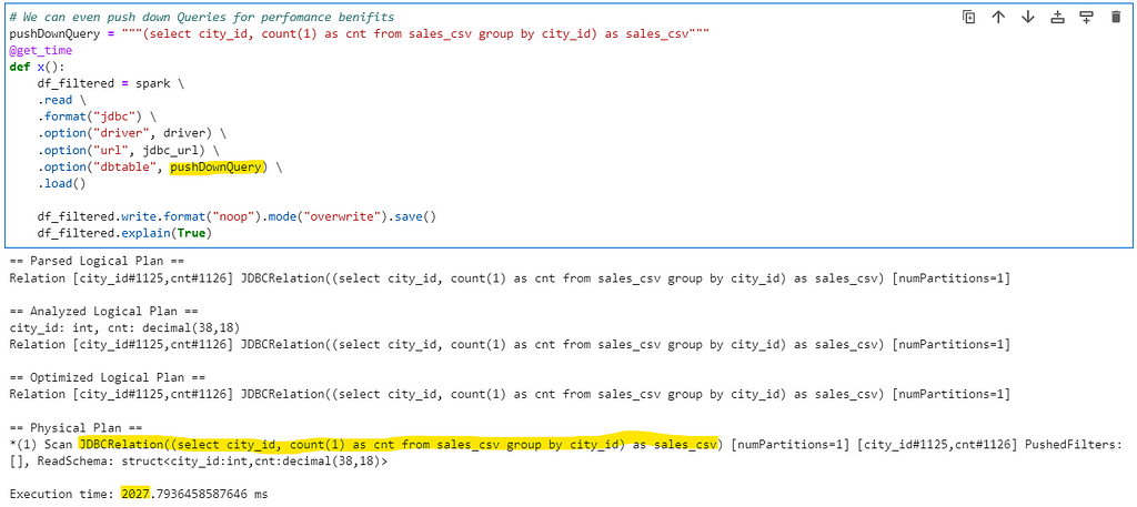
Spark pushes the query to Physical plan, treats the same as table, executes in database and then reads the data.

Bonus tip: While reading data using JDBC and using cache(), be very careful, else it will cripple the Physical plan and Predicates will not be pushed. Check the example below

# Cripple the performance for Predicate Pushdown
@get_time
def x():
    df_filtered = spark \
    .read \
    .format("jdbc") \
    .option("driver", driver) \
    .option("url", jdbc_url) \
    .option("dbtable", table_name) \
    .load() \
    .cache() \
    .filter("city_id = 216510442")
    
    df_filtered.write.format("noop").mode("overwrite").save()
    df_filtered.explain(True)

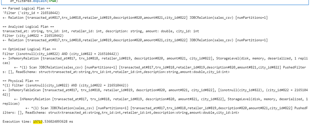
Spark reads all data and cache it. The predicates are applied to cached data later, thus crippling the Predicate Pushdown.

Conclusion: In case of reading data from JDBC sources make sure to push the filter as soon as possible to optimize the performance.

Checkout the iPython notebook on Github — https://github.com/subhamkharwal/ease-with-apache-spark/blob/master/15_JDBC_Predicate_Pushdown.ipynb

Follow my personal blog — https://urlit.me/blog/

Checkout the PySpark Series on Medium — https://subhamkharwal.medium.com/learnbigdata101-spark-series-940160ff4d30

Wish to Buy me a Coffee: Buy Subham a Coffee