URLit.me Blogs

Data Lakehouse with PySpark — Batch Loading Strategy

In this article we are going to design the Batch Loading Strategy to load data in our Data Lakehouse for the series Data Lakehouse with PySpark. This is a well-known and re-usable strategy which can be implemented as a part any Data Warehouse or Data Lakehouse project.

If you are new to Data Lakehouse checkout — https://youtube.com/playlist?list=PL2IsFZBGM_IExqZ5nHg0wbTeiWVd8F06b

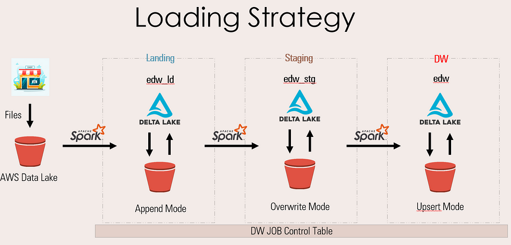
We broke down the complete architecture of the Data Lakehouse into three parts/layers — Landing, Staging and DW.

There are few basic rules for data population for all three layers, lets check them out.

Landing Layer

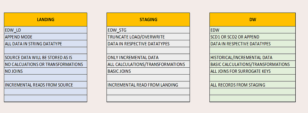
The landing layer will hold the extracted source data. The data will be inserted into the landing table always in APPEND mode with insert_dt and update_dt as audit column.

The value for these audit columns is the current_timestamp when the data is written to the layer. It will help us to read only the incremental data to the subsequent layers.

Also, we will cast all data to string datatype in landing to store the data as is. There will be no joining of tables or any transformation of data in this layer. This layer is strictly to hold Source data which will help us to debug any failures due to data issue.

Staging Layer

The Staging layer will extract the incremental data from the Landing layer based on the insert_dt/update_dt audit columns of the landing table. Data will always be written in OVERWRITE mode.

All transformations and joins required for calculations will be done on this layer and this is main the reason for Overwrite mode, so to have only incremental data in the layer which will help in faster operations.

Data will be finally casted to its final datatype as per DW design. The Staging table will also resemble to final DW table except for the Surrogate Key columns.

DW Layer

The final DW layer will extract all data from Staging and transform for Surrogate Key population. The joins in this layers will be majorly for Surrogate Key population in Facts. All major calculations/transformations will be part of Staging Layer.

Finally the data will be written to respective Dimension or Fact tables as per the requirement of SCDs or Append modes.

Summary for all layers

To support all the incremental and full load scenarios we have an extra element called — JOB Control table, which will hold status and the timestamp for all pipeline execution. It will also be part of filter conditions to incremental data extracts (we will see this as part of demo is future article).

Note: Since the pipelines are broken down into multiple layers, we have a benefit of Fault tolerance as well. In case of any failure, we can just restart pipeline for that layer. And this also helps in parallelizing the loads to multiple layers altogether.

Checkout the following YouTube video, to understand in elaboration

Make sure to Like and Subscribe.

Follow us on YouTube: https://youtube.com/@easewithdata

Checkout the complete Data Lakehouse series on YouTube — https://youtube.com/playlist?list=PL2IsFZBGM_IExqZ5nHg0wbTeiWVd8F06b